
🛢️🤖 Inferring Pipeline State: Using Hidden Markov Models to Reduce False Leak Alarms
Disclaimer:
Hidden Markov Models were new territory for me, and understanding the underlying math required building the forward, backward, and Viterbi procedures from scratch in NumPy. While I’ve developed a much stronger intuition for how the parameters λ = (A, B, π) drive inference, I’m still refining my understanding. This post reflects what worked in our environment and what I’ve learned so far.
This post is a follow-up to 🛢️🤖 Why Detecting O&G Pipeline Anomalies Is So Hard, where I discussed the technical complexity we encountered while building a capability to ingest PI historian data into Databricks for further processing.
Use Case
The technical work is driven by one core objective: reduce unnecessary pipeline shutdowns caused by false leak alarms. In many cases, these shutdowns are not caused by true failures, but by conservative safety mechanisms reacting to limited visibility into the true state of the pipeline and incomplete or uncertain system context. A common pain point is how operational slack is assessed. Controllers often must manually estimate slack conditions in real time, without a fully observable view of packing or unpacking behavior across the line. It’s error-prone and easy to miss during high-pressure operations. When slack is misjudged (or missed entirely), monitoring systems can trigger false leak or deviation alarms, leading to avoidable shutdowns and unnecessary investigations.
To address these challenges, we developed the Deviation Counter Tool to work hand-in-hand with our pipeline state detection. When the ML model infers that the pipeline has entered a specific state, such as unpacking (i.e., shutting down), the deviation counter logic is automatically activated. This tool continuously monitors for deviations, removing the need for manual slack estimation and reducing the risk of false alarms.
Key Terms: Slack, Pack, and Unpack
- Slack: The presence of unpressurized or low-pressure sections in a pipeline, often due to imbalances between inflow and outflow. Slack can lead to inaccurate flow measurements and complicate leak detection.
- Pack (Packing): The process of increasing pressure in the pipeline by introducing more product (inflow exceeds outflow), typically during startup or ramp-up operations.
- Unpack (Unpacking): The process of decreasing pressure in the pipeline by reducing inflow or increasing outflow (outflow exceeds inflow), often during shutdown or ramp-down operations.
Data Ingestion
Everything starts with data engineering. None of the reporting, analytics, or ML happens without it. We are leveraging the PI Web API to pull a subset of PI tags from our meters. Specifically:
- Inflow (product entering a meter)
- Outflow (product leaving a meter)
- Over/short (outflow minus inflow, where a negative value indicates potential loss or leak)
We’re ingesting 1-minute data every 3–5 minutes into our data lake and exposing the tables in Unity Catalog for dashboarding and machine learning.
A lot of effort has gone into hardening this ingestion pipeline.
We’re also running a data quality engine during ingestion. For example, we explicitly check for stale SCADA records. If a DQ issue is detected, we flag it and ignore the data in our ML model for state prediction. We don’t want to generate predictions off poor-quality historian data.
Machine Learning Approach
In the previous blog, I talked about potentially approaching this use case as a classification problem. We are still considering that approach, potentially leveraging something like a nearest neighbor algorithm, and modeling different pipeline states (i.e., normal, shutdown, leak). However, we have had some recent success using a Hidden Markov Model (HMM). In fact, there’s relevant academic work that inspired this direction from the College of Science, Engineering, and Technology in Houston. In ‘Hidden Markov Models for Pipeline Damage Detection Using Piezoelectric Transducers’, researchers applied an HMM-based method to detect pipeline leaks and crack conditions by mapping different damage conditions to distinct Markov states and using statistical signal features as the observable emissions. Their method showed that a Gaussian mixture model HMM (GMM-HMM) could successfully recognize whether a pipeline had a leak, and in some cases, locate it under time-varying conditions, despite noisy measurements.
HMMs can be useful for handling sequential data where the underlying process isn’t directly visible, but you can infer it from patterns in the observations. They typically excel in noisy, time-series environments because they account for uncertainty and temporal dependencies. The HMM is based on a Markov chain, which is a model that tells us something about the probabilities of sequences of random variables (states), each of which can take on values from some set. Hidden Markov Models are designed specifically for sequential data where the true state is not directly observable. That description fits pipeline operations almost perfectly.
From Weather to Pipelines: A Markov Perspective
The classic example for HMMs is the “weather example”:
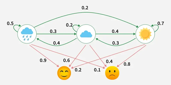
In this diagram:
- Hidden states: Weather conditions (Rainy, Cloudy, Sunny)
- Observations: Emotions (Happy, Neutral, Sad)
- Green arrows: Transition probabilities, the likelihood the weather changes from one state to another each day
- Red arrows: Emission probabilities, the likelihood of observing a particular emotion given the current weather
We only see the emotions (observations), not the weather (hidden states). The HMM helps infer the most likely sequence of hidden states behind those observations.
The same idea applies to pipelines.
Observable data (what we measure):
- Inflow
- Outflow
- Over/short
Hidden states (what we actually care about):
- Normal operation
- Line packing (starting up)
- Line unpacking (shutting down)
- Leak
- Shutdown
- Transition states
An HMM asks a more realistic question:
“Given everything we’ve observed up to now, what state are we most likely in, and how likely is it to transition to another state?”
That temporal dependency is critical because pipeline states persist. A leak doesn’t appear and disappear randomly minute to minute. A line doesn’t pack instantly. Modeling persistence reduces noise-driven false positives.
This model is a multivariate Gaussian HMM (one Gaussian per state) with 6 hidden states and diagonal covariance, trained unsupervised on 9 standardized, flow-derived features (inflow, outflow, over/short, ratios, deltas, and operational flags).
The HMM was trained and versioned within Unity Catalog, and it took nine iterations to align the transition structure and feature engineering with operational reality. I’m sure many more iterations are ahead as we collect more data, observe edge cases, and continue refining how the model reflects real pipeline behavior.
We leveraged tools like StandardScaler to account for unit variance, and engineered features for flow relationships (e.g., inflow/outflow ratio), temporal dynamics (e.g., delta inflows & outflows based on a lag window), and operational flags (e.g., binary flag for inflow < 5.0 (shutdown detection)).
Orchestration & Deployment
All our artifacts in Databricks from ingestion of the PI data to predicting pipeline state via batch inference leveraging the HMM, are deployed via asset bundles and orchestrated in workflows.
We are also leaning heavily on Unity Catalog to version our HMM, so we have version history for training iterations.
Conclusion
One challenge we’ve run into is temporal resolution.
We’re currently ingesting 1-minute data every 3–5 minutes. That sounds reasonable until you see something like this:
| Time | Inflow | Outflow |
|---|---|---|
| 1:00 | 236 | 343 |
| 1:01 | 0 | 0 |
At first glance, everything looks within range… and then it drops to zero.
We pulled second-by-second data for that same window to see what happened in those 60 seconds.
Apparently, a lot can happen in 60 seconds in pipeline operations.
We may need to increase ingestion frequency because pulling at a minute granularity can miss critical context. When you’re modeling state transitions, that missing context matters.
There is still a lot to learn, but we’re getting closer to something that reflects operational reality rather than just reacting to noisy signals.
Big shoutout to Shawn for helping sharpen how we framed the operational problem, and to Mark for leading the data engineering effort that makes any of this possible.
Thanks for reading! 😀